Every feature
One part, one frame, one decision — and everything that comes after
A camera sees the part, a model decides in under 100 ms, and the machine acts on it. What makes the system worth having is what happens next: every image kept, every defect classified, every pattern findable.
Capture
It starts with the frame
No model recovers a defect the optics never resolved. Getting the camera, the lens and the light right for your part is the first half of the job, and it is where a project starts.
Industrial cameras, matched to the part
Machine vision cameras selected for resolution, sensor size and interface — not a fixed bundle. Global shutter for parts in motion, resolution chosen so the smallest defect you care about lands on enough pixels to be segmented.
Several angles on the same part
Most parts need more than one view. Multiple cameras trigger together on the same part and their results are combined into one verdict, so a part is only accepted when every angle agrees.
Triggered by the machine
The system takes its trigger from the line — robot position, ejector, encoder or PLC signal — so images are captured at the same point in the cycle every time. Consistent framing is what makes the data comparable later.
Optics you can calculate before you buy
Working distance, field of view, focal length and pixels per millimetre worked out up front.
A camera database, not a catalogue
Sensor specs, resolution, frame rate and interface for the cameras we work with, filterable against what your part needs.
Decide
The decision happens at the machine
Inference runs on a GPU box in the cabinet next to the line. Nothing waits on a network round trip, and nothing stops if the connection does.
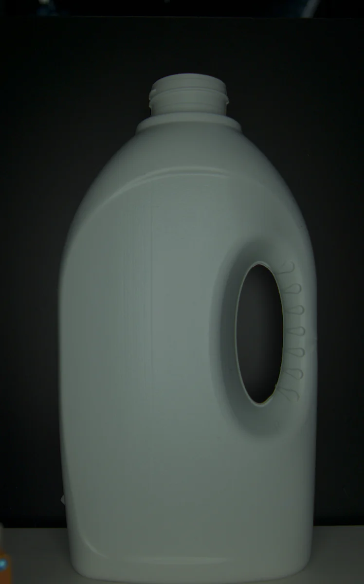
The defects that matter on a moulding line, on real parts
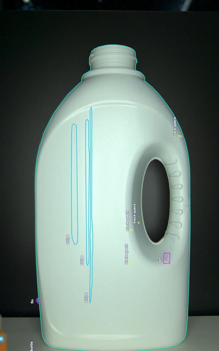
- Bottle
- Stripe
- Black speck
- Dirt
- Fin
Surface level defects
One frame, many questions answered at once. The model segments the bottle itself, then every stripe, black speck and patch of dirt on it — each as an outline rather than a box. An outline can be measured, so the same pass that finds a defect also classifies it, sizes it in mm², and decides whether it crosses the threshold that fires the reject.
Edge compute sized to the line
Our fastest models return a verdict within 80 ms per image, measured on one camera, fast enough for lines producing thousands of parts an hour. Where cycle time allows, the same models run on smaller, cheaper compute — the hardware is matched to the throughput, not sold by default.
Segmentation
The one we reach for most. Every defect comes back as a pixel-accurate outline rather than a box, which means it can be measured, sized in mm² and thresholded individually.
Classification
Accept or reject against a defined set of defect types, or confirm that everything that should be present is present.
Object detection
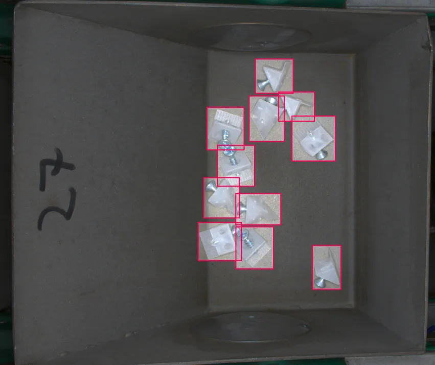
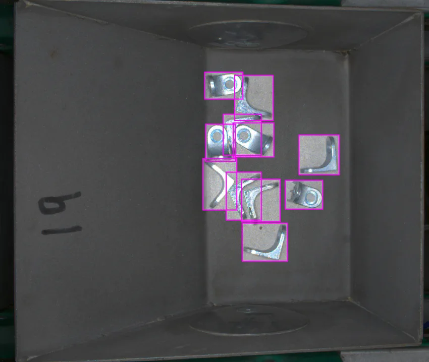
Find and count parts regardless of how they lie. Used where weighing and counting sensors fail, including mixed SKUs in random orientation.
Measurement
Dimensional checks read off the segmentation mask, in millimetres, against tolerance.
Thresholds you set, per class
A stripe of 2 mm² and a stripe of 20 mm² are not the same problem. Because every detection is measured, you decide per defect class what passes, what is flagged and what fires the reject — rather than accepting a single global sensitivity.
Cavity marks read from the part
Where the tool marks the cavity number, the system reads it and attaches it to the record. This is what turns a reject into a lead on the tool.
Act
A verdict is only useful if the line can use it
The output is a signal your equipment already understands, at the moment it needs it.
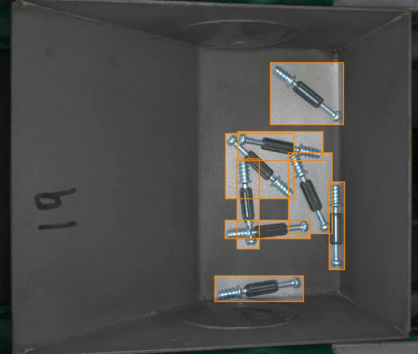
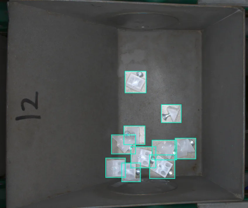
Live view at the machine
What the operator sees, right now. Detections drawn on the stream as parts pass, with cavity, class and confidence attached, and a running list of recent inspections.
Reject signalling
A digital output on the verdict, timed to the cycle, driving whatever the line uses to separate the part — ejector, blow-off, diverter, or a robot that stacks good parts and sets the rejects aside.
MQTT and PLC integration
Results are published over MQTT today. Function libraries for the common PLC platforms are in development, so your integrator will write the line logic in the environment they already work in. We deliver the camera and the model; the automation stays where it belongs.
Built for the operator, not the data scientist
The screen at the machine answers one question — what was wrong with that part, and which cavity did it come from — without anyone opening a training tool.
Record
Every part inspected, every image kept
The value compounds after the first week. A rejected part that leaves no trace teaches you nothing; a rejected part with an image, a class, a size, a cavity and a timestamp is data.
Production runs
Go back to any run and see what was produced and what the system caught — part, batch, start time, parts inspected, NOK count and reject rate.
| Run | Part | Batch | Started | Parts | NOK | Rate | |
|---|---|---|---|---|---|---|---|
| R-4821 | Cap 32mm | B-2291 | 08.03 07:02 | 18,420 | 61 | 0.33% | Completed |
| R-4820 | Lid 88mm | B-2288 | 07.03 23:04 | 21,150 | 44 | 0.21% | Completed |
| R-4819 | Cap 32mm | B-2287 | 07.03 15:01 | 19,880 | 96 | 0.48% | Flagged |
| R-4818 | Housing A | B-2284 | 07.03 07:03 | 16,240 | 38 | 0.23% | Completed |
The image archive
Every image that passed through the model is stored with its predictions, browsable by run, by date, by confidence or by defect count. When an operator catches a defect the system missed, you narrow to the time window and pull the exact frames.
Traceability by batch and part
Inspection records tied to part number and batch, so a customer question about a specific delivery has an answer with images behind it.
Documentation and reporting
Run-level and period-level reporting, exportable for internal quality review or for a customer audit.
Understand
From “a part failed” to “here is why”
Once every defect carries a class, a size and a place in the process, patterns surface on their own: which cavity, which shift, which material batch. That is the difference between knowing your reject rate and knowing what causes it.
Defects by cavity
The single most actionable view. Black specks concentrated in cavity 1 and warping concentrated in cavity 4 are two different tool problems, and neither is visible in an aggregate reject rate.
Defects over time
Reject rate by hour, by shift and by run. Sudden steps point at a changeover, a material batch or a setting; slow drift points at wear.
Breakdown by defect class
Which faults dominate, and how the mix changes — so improvement effort goes where the volume is.
Dimensional tolerance
Share of parts within tolerance, over and under, tracked continuously rather than sampled.
A risk view
Frequency weighted against how confident the model is, so the defects that are both common and certain rise to the top of the list.
Ask it in plain language
A statistics assistant over your own inspection data — ask what changed last night or which cavity is worst this week and get the answer without building a query.
Improve
The model gets better because your line runs
A vision system that is frozen at commissioning starts drifting the day the product changes. This one is built to be retrained by the people who own it.
Find the weak spots by confidence
Sort any run by lowest confidence and you see exactly where the model is unsure — a particular defect type, a particular orientation, a particular corner of the frame. Those are the images worth re-annotating.
Annotate and correct
Fix the masks, add the class that was missing, upload new images from your computer or straight from the cameras on the line. Datasets are versioned, so you can always see which data produced which model.
Retrain in the cloud, deploy to the machine
Pick a dataset version, set the training running, and a few hours later you have a new model to deploy to the box on the line. The line keeps running on the current model throughout.
A route for new colours, labels and variants
When a new variant enters production, the first run captures images while the parts are checked as they are today. Those images become training data, and the variant runs under full inspection from the next order onward. Over time the model generalises across variants instead of needing one model per SKU.
First step
Prove the defects are detectable
You send 100 parts — 50 good, 50 faulty. We photograph them, train a model on them in our lab, and 14 days later you have the report.
What the report contains — click a page
Guarantee
If we cannot find the defect type you point at, you get your money back. Buy the system within 60 days and the fee is credited in full.
DKK 8,000